Theory and Implementation of GroundwaterDupuitPercolator#

Governing Equations#

Variably-saturated groundwater flow is often assumed to be governed by the Richards equation, which describes how water content and/or total energy potential evolve in an idealized porous medium due to fluxes of water driven by gradients in total potential, \(h = z + p/ \gamma\), where \(z\) is the elevation head, \(p\) is the gage pressure, and \(\gamma\) is the specific weight of water.

\[\frac{\partial \theta}{\partial t} = \frac{\partial}{\partial x} \bigg( k \frac{\partial h}{\partial x} \bigg) + \frac{\partial}{\partial y} \bigg( k \frac{\partial h}{\partial y} \bigg) + \frac{\partial}{\partial z} \bigg( k \frac{\partial h}{\partial z} \bigg)\]

Here \(\theta\) is the volumetric water content of the aquifer and \(k\) is the hydraulic conductivity, which may be a function of \(\theta\). Here we use the widely applied Dupuit-Forcheimer approximation, which is valid when the aquifer is laterally extensive in comparison to its thickness, and the capillary fringe above the water table is relatively thin. If this is the case, the component of the hydraulic gradient normal to the aquifer base can be neglected, and the water table can be treated as a free surface. Consequently, the total head is equal to the water table elevation, \(h=z\). With these assumptions, an adjusted governing equation can be written for the time evolution of the water table elevation:

\[n \frac{\partial h}{\partial t} = \frac{\partial}{\partial x} \bigg( k_{sat} h \frac{\partial h}{\partial x} \bigg) + \frac{\partial}{\partial y} \bigg( k_{sat} h \frac{\partial h}{\partial y} \bigg)\]

where \(n\) is the drainable porosity, and \(k_{sat}\) is the saturated hydraulic conductivity.

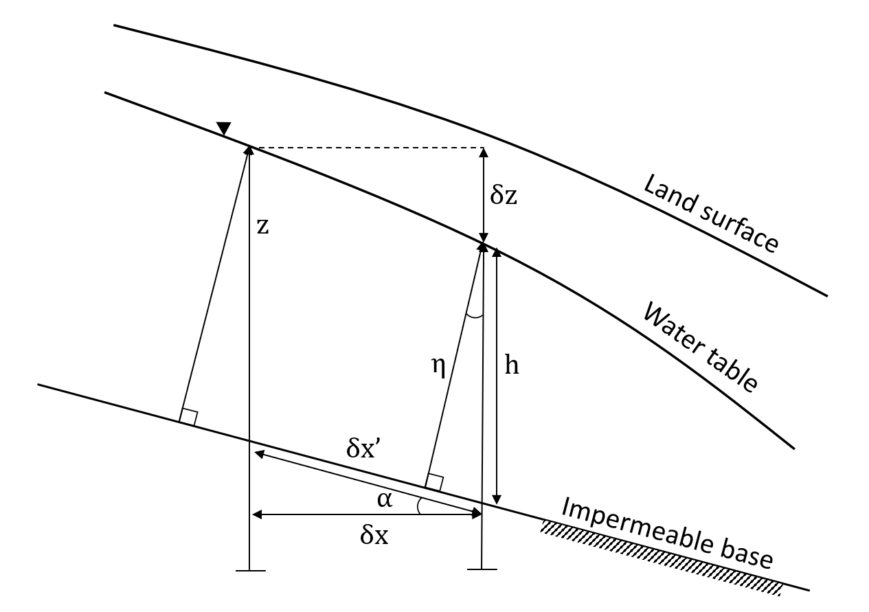
Aquifer schematic. — Aquifer schematic showing vertical aquifer thickness \(h\), bed-normal aquifer thickness \(\eta\), and water table elevation \(z\).#

When the aquifer base is sloping, the governing equations must be adjusted. Childs (1971) provides the governing equation for the groundwater specific discharge as:

\[q_{x'} = - k_{sat} \eta \frac{\partial z}{\partial x'}\]

where \(x'\) is the coordinate parallel to the impermeable base, and \(\eta\) is the aquifer thickness perpendicular to the impermeable base ([2]). The GroundwaterDupuitPercolator treats two additional fluxes that affect aquifer storage: groundwater return flow to the surface \(q_s\), and recharge from precipitation \(f\). Implementations of the Dupuit-Forcheimer model often encounter numerical instabilities as the water table intersects the land surface. To alleviate this problem, we use the regularization approach introduced by Marcais et al. (2017), which smooths the transition between surface and subsurface flow ([1]). The complete governing equations in the base-parallel reference frame \((x',y')\) are:

\[\begin{split}\begin{aligned} n \frac{\partial \eta}{\partial t} &= f \cos(\alpha) - q_s \cos(\alpha) - \nabla' \cdot q \\ q &= -k_{sat} \eta \big( \nabla' z ) \\ q_s &= \mathcal{G}_r \bigg( \frac{\eta}{d'} \bigg) \mathcal{R} \big(-\nabla' \cdot q + f \cos(\alpha) \big) \\\end{aligned}\end{split}\]

where \(\alpha\) is the slope angle of aquifer base, and \(d'\) is the permeable thickness normal to the aquifer base. The gradient operator \(\nabla'\) and divergence operator \(\nabla' \cdot\) are calculated with respect to the base-parallel coordinate system. Note that the surface runoff is the sum of both groundwater return flow and precipitation on saturated area.

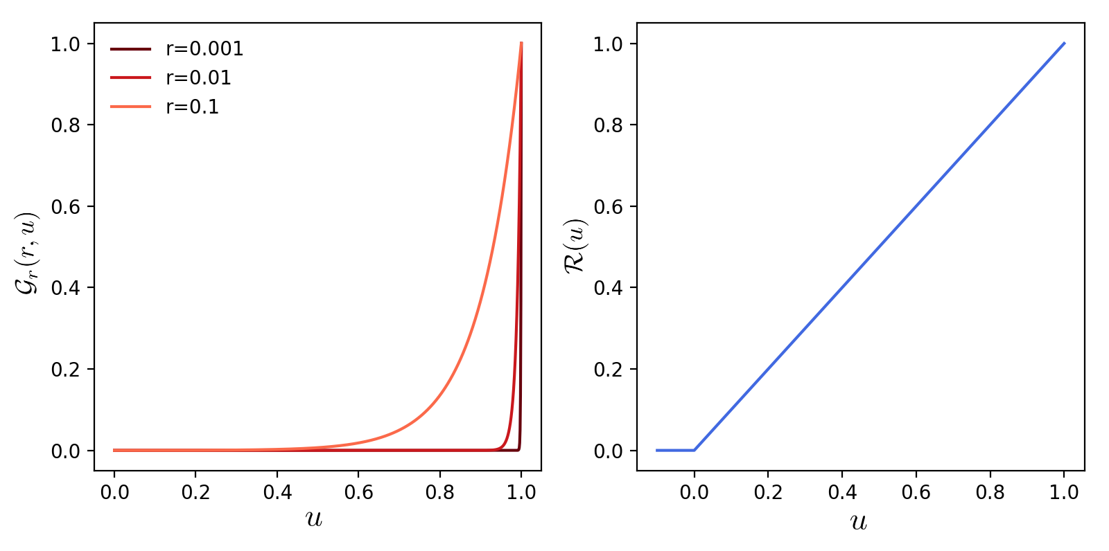
The expression for \(q_s\) utilizes two regularization functions \(\mathcal{G}_r\) and \(\mathcal{R}\):

\[\mathcal{G}_r(r,u) = \exp \bigg( - \frac{1-u}{r} \bigg)\]

\[\mathcal{R}(u) = u \mathcal{H}(u)\]

where \(r\) is a user-specified regularization factor and \(\mathcal{H}(u)\) is the Heaviside step function:

\[\begin{split}\mathcal{H}(u) = \left\{ \begin{array}{ll} 0 & u<0 \\[8pt] 1 & u \geq 0 \end{array} \right.\end{split}\]

To recast the problem in terms of the horizontal coordinate system used by Landlab, we make the substitutions \(\eta = h \cos(\alpha)\), \(x = x' \cos(\alpha)\), and \(y = y' \cos(\alpha)\). In the horizontal coordinate system \((x,y)\), the governing equations are:

\[\begin{split}\begin{aligned} n \frac{\partial h}{\partial t} &= f - q_s - \nabla \cdot q \\ q &= -k_{sat} \cos^2(\alpha) h \big( \nabla z ) \\ q_s &= \mathcal{G}_r \bigg( \frac{h}{d} \bigg) \mathcal{R} \big(f - \nabla \cdot q \big) \\\end{aligned}\end{split}\]

where \(d\) is the vertical regolith thickness, and the gradient operator \(\nabla\) and divergence operator \(\nabla \cdot\) are calculated with respect to the horizontal coordinate system \((x,y)\).

Numerical Implementation#

We use an explicit, forward-in-time finite-volume method to solve the governing equations. In this method, gradients are calculated at links (between volume centers), and flux divergences are calculated at nodes (at volume centers). The governing equation with timestep \(\Delta t\) is:

\[n \bigg( \frac{h^{t+\Delta t} - h^t}{\Delta t} \bigg) = f^t - q_s^t - \nabla \cdot q^t\]

Below is a description of the components needed to calculate the right side of this equation. To calculate the groundwater flux \(q\), the gradients of aquifer base elevation \(b\) and water table elevation \(z\) must be determined. The slope angle of the aquifer base is calculated from the aquifer base elevation \(b\):

\[\begin{split}\begin{aligned} \alpha_{ij} =& \arctan \big( (\nabla b)_{ij} \big) \\ \big( \nabla b \big)_{ij} =& \frac{b_{i} - b_{j}}{L_{ij}}\end{aligned}\end{split}\]

where the subscripts \(i\) and \(j\) indicate the nodes at the head and tail of the link respectively, and \(L_{ij}\) is the length of the link. The gradient \(\nabla z\) is calculated on link \(ij\) as:

\[\big( \nabla z \big)_{ij} = \frac{z_{i} - z_{j}}{L_{ij}}\]

Flux divergence is calculated by summing the fluxes into an out of the links that connect to a node. The divergence of the groundwater flux is:

\[\big( \nabla \cdot q \big)_i = \frac{1}{A_i} \sum_{j \in S} \delta_{ij} q_{ij} \lambda_{ij}\]

where \(A_i\) is the area of node \(i\), \(S\) is the set of nodes that have links that connect to node \(i\), and \(\delta_{ij}\) is a function that is equal to +1 if the link points away from the node (the tail of the link is at node \(i\)), and equal to -1 if the link points toward the node (the head of the link is at node \(i\)). The groundwater flux on the link is \(q_{ij}\) and the width of the face through which \(q_{ij}\) passes is \(\lambda_{ij}\).

References: