Introduction to Landlab’s Gridding Library#

When creating a two-dimensional simulation model, often the most time-consuming and error-prone task involves writing the code to set up the underlying grid. Irregular (or “unstructured”) grids are especially tricky to implement. Landlab’s ModelGrid package makes this process much easier, by providing a set of library routines for creating and managing a 2D grid, attaching data to the grid, performing common input and output operations, and providing library functions that handle common numerical operations such as calculating a field of gradients for a particular state variable. By taking care of much of the overhead involved in writing grid-management code, ModelGrid is designed to help you build 2D models quickly and efficiently, freeing you to concentrate on the science behind the code.

Some of the things you can do with ModelGrid include:

Create and configure a structured or unstructured grid in a one or a few lines of code
Create various data arrays attached to the grid
Easily implement staggered-grid finite-difference/finite-volume schemes
Calculate gradients in state variables in a single line
Calculate net fluxes in/out of grid cells in a single line
Set up and run “link-based” cellular automaton models
Switch between structured and unstructured grids without needing to change the rest of the code
Develop complete, 2D numerical finite-volume or finite-difference models much more quickly and efficiently than would be possible using straight C, Fortran, Matlab, or Python code

Some of the Landlab capabilities that work with ModelGrid to enable easy numerical modeling include:

Easily read in model parameters from a formatted text file
Write grid and data output to netCDF files for import into open-source visualization packages such as ParaView and VisIt
Create grids from ArcGIS-formatted ascii files
Create models by coupling together your own and/or pre-built process components
Use models built by others from process components

This document provides a basic introduction to building applications using Landlab’s ModelGrid. It covers: (1) how grids are represented, and (2) a set of tutorial examples that illustrate how to build models using simple scripts.

How a Grid is Represented#

Basic Grid Elements#

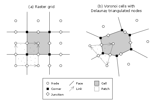
../_images/grid_schematic_ab.png — *Figure 1*: Elements of a model grid. The main grid elements are nodes, links, cells, and faces. Less commonly used elements include corners, patches, and junctions. In the spring 2015 version of Landlab, **ModelGrid** can implement raster (a) and Voronoi-Delaunay (b) grids. Ordered subtypes of Voronoi-Delaunay grids—radial and hexagonal—are also available. (Note that not all links and patches are shown, and only one representative cell is shaded.)#

Figure 1 illustrates how ModelGrid represents a simulation grid. The grid contains a set of (x,y) points called nodes. In a typical finite-difference or finite-volume model, nodes are the locations at which one tracks scalar state variables, such as water depth, land elevation, sea-surface elevation, or temperature.

Each adjacent pair of nodes is connected by a line segment known as a link. A link has both a position in space, denoted by the coordinates of the two bounding nodes, and a direction: a link runs from one node (known as its from-node or tail-node) to another node (known as its to-node or head-node).

Every node in the grid interior is associated with a polygon known as a cell (illustrated, for example, by the shaded square region in Figure 1a). Each cell is bounded by a set of line segments known as faces, which it shares with its neighboring cells.

In the simple case of a regular (raster) grid, the cells are square, the nodes are the center points of the cells (Figure 1), and the links and faces have identical length (equal to the node spacing). In a Voronoi-Delaunay grid, the cells are Voronoi polygons (also known as Theissen polygons) (Figure 1a). In this case, each cell represents the surface area that is closer to its own node than to any other node in the grid. The faces represent locations that are equidistant between two neighboring nodes. Other grid configurations are possible as well. The spring 2015 version of Landlab includes support for hexagonal and radial grids, which are specialized versions of the Voronoi-Delaunay grid shown in Figure 1a. Note that the node-link-cell-face topology is general enough to represent other types of grid; for example, one could use ModelGrid’s data structures to implement a quad-tree grid, or a Delaunay-Voronoi grid in which cells are triangular elements with nodes at their circumcenters.

Creating a Grid#

Creating a grid is easy. The first step is to import Landlab’s RasterModelGrid class (this assumes you have installed Landlab)

>>> from landlab import RasterModelGrid

Now, create a regular (raster) grid with 10 rows and 40 columns, with a node spacing (dx) of 5:

>>> mg = RasterModelGrid((10, 40), 5.0)

mg is now a grid object with 400 ( 10*40 ) nodes and 750 ( 40*(10-1) + 30*(10-1) ) links.

>>> mg.number_of_node_columns
40
>>> mg.number_of_nodes
400
>>> mg.number_of_links
750

Adding Data to a Landlab Grid Element using Fields#

Landlab has a data structure called fields that will store data associated with different types of grid elements. Fields are convenient because 1) fields create data arrays of the proper length for the associated grid element, and 2) fields attach these data to the grid, so that any piece of code that has access to the grid also has access to the data stored in fields.

Suppose you would like like to track the elevation at each node. The following code creates a data field (array) called elevation. In this case, we’ll use the grid method add_zeros to create a field that initially sets all values in the field to zero (we’ll explain how to read in elevation values from a file in the section on DEMs below). The add_zeros method takes two arguments: the name of the grid element (in this case, node, in the singular) and a name we choose for the value in the data field (here we’ll just call it elevation). Each elevation value in the data field is then associated with a specific grid node. The data field is just a NumPy array whose length is equal to the number of nodes in the grid.

>>> z = mg.add_zeros("elevation", at="node")

Here z is an array of zeros. We can verify that z has the same length as the number of nodes:

>>> z.size  # or len(z)
400

Note that z is a reference to the data stored in the model field. This means that if you change z, you also change the data in the ModelGrid’s elevation field. Therefore, you can access and manipulate data in the field either through the variable z or through the grid, as in the following examples:

>>> mg.at_node["elevation"][5] = 1000.0

or the alternative notation:

>>> mg["node"]["elevation"][5]
1000.

Now the sixth element in the model’s elevation field array, or in z, is equal to 1000. (Remember that the first element of a Python array has an index of 0 (zero)).

You can see all of the field data available at the nodes on mg with the following:

>>> mg.at_node.keys()
['elevation']

You may recognize this as a dictionary-type structure, where the keys are the names (as strings) of the data arrays.

There are currently no data values (fields) assigned to the links, as shown by the following:

>>> mg.at_link.keys()
[]

It is also possible, and indeed, often quite useful, to initialize a field from an existing NumPy array of data. You can do this with the add_field method. This method allows slightly more granular control over how the field gets created. In addition to the grid element and field name, this method takes an array of values to assign to the field. Optional arguments include: units= to assign a unit of measurement (as a string) to the value, copy= a boolean to determine whether to make a copy of the data, and clobber= a boolean that prevents accidentally overwriting an existing field.

>>> import numpy as np
>>> elevs_in = np.random.rand(mg.number_of_nodes)
>>> mg.add_field(
...     "elevation", elevs_in, at="node", units="m", copy=True, clobber=True
... )

Fields can store data at nodes, cells, links, faces, patches, junctions, and corners (though the latter two or three are very rarely, if ever, used). The grid element you select is described in Landlab jargon as that field’s centering or group, and you will sometimes see these terms used as input parameters to various grid methods.

To access only the core nodes, core cells, active links, or some other subset of node values using the properties available through the ModelGrid, you can specify a subset of the field data array. For example, if we wanted to determine the elevations at core nodes only we can do the following:

>>> core_node_elevs = mg.at_node["elevation"][mg.core_nodes]

The first set of brackets, in this case elevation, indicates the field data array, and the second set of brackets, in this case mg.core_nodes (itself an array of core node IDs), is a NumPy filter that specifies which elevation elements to return.

Here is another example of initializing a field with the add_ones method. Note that when initializing a field, the singular of the grid element type is provided:

>>> veg = mg.add_ones("percent_vegetation", at="cell")
>>> mg.at_cell.keys()
['percent_vegetation']

Here veg is an array of ones that has the same length as the number of cells. Because there are no cells around the edge of a grid, there are fewer cells than nodes:

>>> mg.at_cell["percent_vegetation"].size
304

As you can see, fields are convenient because you don’t have to keep track of how many nodes, links, cells, etc. there are on the grid. It is easy for any part of the code to query what data are already associated with the grid and operate on these data.

You are free to call your fields whatever you want. However, field names are more useful if standardized across components. If you are writing a Landlab component you should use Landlab’s standard names. Standard names for fields in a particular component can be accessed individually through the properties component_instance._input_var_names and component_instance._output_var_names (returned as dictionaries), and are listed in the docstring for each component.

>>> from landlab.components.flexure import Flexure
>>> flexer = Flexure(rg)
>>> flexer._input_var_names
{'lithosphere__elevation',
 'lithosphere__overlying_pressure',
 'planet_surface_sediment__deposition_increment'}
>>> flexer._output_var_names
{'lithosphere__elevation', 'lithosphere__elevation_increment'}

We also maintain this list of all the Landlab standard names.

Our fields also offer direct compatibility with CSDMS’s standard naming system for variables. However, note that, for ease of use and readability, Landlab standard names are typically much shorter than CSDMS standard names. We anticipate that future Landlab versions will be able to automatically map from Landlab standard names to CSDMS standard names as part of Landlab’s built-in Basic Model Interface for CSDMS compatibility.

The following gives an overview of the commands you can use to interact with the grid fields.

Field initialization#

grid.add_empty(name, at="group", units="-")
grid.add_ones(name, at="group", units="-")
grid.add_zeros(name, at="group", units="-")

“group” is one of ‘node’, ‘link’, ‘cell’, ‘face’, ‘corner’, ‘junction’, ‘patch’

“name” is a string giving the field name

“units” (optional) is a string denoting the units associated with the field values.

Field creation from existing data#

grid.add_field(name, value_array, at="group", units="-", copy=False, clobber=True)

Arguments as above, plus:

“value_array” is a correctly sized numpy array of data from which you want to create the field.

“copy” (optional) if True adds a copy of value_array to the field; if False, creates a reference to value_array.

“clobber” (optional) if False, raises an exception if a field called name already exists.

Field access#

grid.at_node or grid['node']
grid.at_cell or grid['cell']
grid.at_link or grid['link']
grid.at_face or grid['face']
grid.at_corner or grid['corner']
grid.at_junction or grid['junction']
grid.at_patch or grid['patch']

Each of these is then followed by the field name as a string in square brackets, e.g.,

>>> grid.at_node["my_field_name"]  # or
>>> grid["node"]["my_field_name"]

You can also use these commands to create fields from existing arrays, as long as you don’t want to take advantage of the added control add_field() gives you.

Getting information about fields#

Landlab offers a command line interface that lets you find out about all the fields that are in use across all the Landlab components. You can find out the following:

$ landlab used_by [ComponentName] # What fields does ComponentName take as inputs?

$ landlab provided_by [ComponentName] # What fields does ComponentName give as outputs?

$ landlab uses [field__name] # What components take the field field__name as an input?

$ landlab provides [field__name] # What components give the field field__name as an output?

$ landlab list # list all the components

$ (landlab provided_by && landlab used_by) | sort | uniq # some command line magic to see all the fields currently used in components

Representing Gradients in a Landlab Grid#

Finite-difference and finite-volume models usually need to calculate spatial gradients in one or more scalar variables, and often these gradients are evaluated between pairs of adjacent nodes. ModelGrid makes these calculations easier for programmers by providing built-in functions to calculate gradients along links and allowing applications to associate an array of gradient values with their corresponding links or edges. The tutorial examples illustrate how this capability can be used to create models of processes such as diffusion and overland flow.

Here we simply illustrate the method for calculating gradients on the links. Remember that we have already created the elevation array z, which is also accessible from the elevation field on mg.

>>> gradients = mg.calculate_gradients_at_active_links(z)

Now gradients have been calculated at all links that are active, or links on which flow is possible (see boundary conditions below).

Other Grid Elements#

The cell vertices are called corners (Figure 1, solid squares <basic_grid_elements>). Each face is therefore a line segment connecting two corners. The intersection of a face and a link (or directed edge) is known as a junction (Figure 1, open diamonds). Often, it is useful to calculate scalar values (say, ice thickness in a glacier) at nodes, and vector values (say, ice velocity) at junctions. This approach is sometimes referred to as a staggered-grid scheme. It lends itself naturally to finite-volume methods, in which one computes fluxes of mass, momentum, or energy across cell faces, and maintains conservation of mass within cells. (In the spring 2015 version of Landlab, there are no supporting functions for the use of junctions, but support is imminent.)

Notice that the links also enclose a set of polygons that are offset from the cells. These secondary polygons are known as patches (Figure 1, dotted). This means that any grid comprises two complementary tesselations: one made of cells, and one made of patches. If one of these is a Voronoi tessellation, the other is a Delaunay triangulation. For this reason, Delaunay triangulations and Voronoi diagrams are said to be dual to one another: for any given Delaunay triangulation, there is a unique corresponding Voronoi diagram. With ModelGrid, one can create a mesh with Voronoi polygons as cells and Delaunay triangles as patches (Figure 1b). Alternatively, with a raster grid, one simply has two sets of square elements that are offset by half the grid spacing (Figure 1a). Whatever the form of the tessellation, ModelGrid keeps track of the geometry and topology of the grid. patches can be useful for processes like calculating the mean gradient at a node, incorporating influence from its neighbors.

Managing Grid Boundaries#

An important component of any numerical model is the method for handling boundary conditions. In general, it’s up to the application developer to manage boundary conditions for each variable. However, ModelGrid makes this task a bit easier by tagging nodes that are treated as boundaries (boundary nodes) and those that are treated as regular nodes belonging to the interior computational domain (core nodes). It also allows you to de-activate (“close”) portions of the grid perimeter, so that they effectively act as walls.

Let’s look first at how ModelGrid treats its own geometrical boundaries. The outermost elements of a grid are nodes and links (as opposed to corners and faces). For example, Figure 2 shows a sketch of a regular four-row by five-column grid created by RasterModelGrid. The edges of the grid are composed of nodes and links. Only the inner six nodes have cells around them; the remaining 14 nodes form the perimeter of the grid.

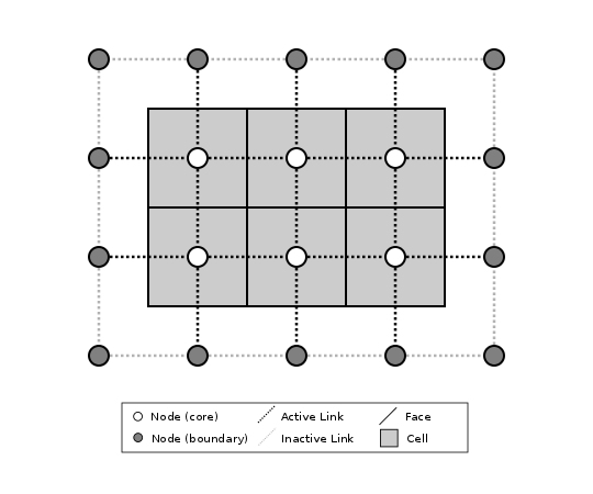
../_images/example_raster_grid.png — Figure 2: Illustration of a simple four-row by five-column raster grid created with `landlab.grid.raster.RasterModelGrid`. By default, all perimeter nodes are tagged as open (fixed value) boundaries, and all interior cells are tagged as core. An active link is one that connects either two core nodes, or one core node and one open boundary node.#

All nodes are tagged as either boundary or core. Those on the perimeter of the grid are automatically tagged as boundary nodes. Nodes on the inside are core by default, but it is possible to tag some of them as boundary instead (this would be useful, for example, if you wanted to represent an irregular region, such as a watershed, inside a regular grid). In the example shown in Figure 2, all the interior nodes are core, and all perimeter nodes are open boundary.

Boundary nodes are flagged as either open or closed, and links are tagged as either active or inactive (Figure 3).

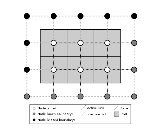
../_images/example_raster_grid_with_closed_boundaries.png — Figure 3: Illustration of a simple four-row by five-column raster grid with a combination of open and closed boundaries.#

A closed boundary is one at which no flux is permitted enter or leave, ever. By definition, all links coming into or out of a closed boundary node must be inactive. There is effectively no value assigned to a closed boundary; it will probably have a grid.BAD_INDEX_VALUE or null value of some kind. An open boundary is one at which flux can enter or leave, but whose value is controlled by some boundary condition rule, updated at the end of each timestep.

An active link is one that joins either two core nodes, or one core and one open boundary node (Figure 3). You can use this distinction in models to implement closed boundaries by performing flow calculations only on active links, as seen in this tutorial.

Boundary condition details and methods#

A call to mg.node_status returns the codes representing the boundary condition of each node in the grid. There are 5 possible types, they are stored on the model grid:

mg.BC_NODE_IS_CORE (Type 0)
mg.BC_NODE_IS_FIXED_VALUE (Type 1)
mg.BC_NODE_IS_FIXED_GRADIENT (Type 2)
mg.BC_NODE_IS_LOOPED (Type 3, used for looped boundaries)
mg.BC_NODE_IS_CLOSED (Type 4)

A number of different methods are available to you to interact with (i.e., set and update) boundary conditions at nodes. Landlab is smart enough to automatically initialize new grids with fixed value boundary conditions at all perimeters and core nodes for all interior nodes, but if you want something else, you’ll need to modify the boundary conditions.

If you are working with a simple Landlab raster where all interior nodes are core and all perimeter nodes are boundaries, you will find useful the set of commands:

mg.set_closed_boundaries_at_grid_edges(right, top, left, bottom)
mg.set_fixed_value_boundaries_at_grid_edges(right, top, left, bottom)
mg.set_fixed_link_boundaries_at_grid_edges(right, top, left, bottom, link_value=None)
mg.set_looped_boundaries(top_bottom_are_looped, left_right_are_looped)

Where right, top, left, bottom are all booleans. See the relevant docstring for each method for more detailed information.

If you are working with an imported irregularly shaped raster grid, you can close nodes which have some fixed NODATA value in the raster using:

mg.set_nodata_nodes_to_closed(node_data, nodata_value)

Note that all of these commands will treat the status of node links as slave to the status of the nodes, as indicated in Figure 3. Links will be set to active or inactive according to what you set the node boundary conditions as, when you call each method.

If you are working on an irregular grid, or want to do something more complicated with your raster boundary conditions, you will need to modify the grid.status_at_node array by hand, using indexes to node IDs. Simply import the boundary types from landlab then set the node statuses. The links will be updated alongside these changes automatically:

>>> grid = RasterModelGrid((5, 5))
>>> grid.set_closed_boundaries_at_grid_edges(False, True, False, True)
>>> grid.number_of_active_links
18
>>> grid.status_at_node[[6, 8]] = mg.BC_NODE_IS_CLOSED
>>> grid.status_at_node.reshape((5, 5))
array([[4, 4, 4, 4, 4],
       [1, 4, 0, 4, 1],
       [1, 0, 0, 0, 1],
       [1, 0, 0, 0, 1],
       [4, 4, 4, 4, 4]], dtype=int8)
>>> grid.number_of_active_links  # links were inactivated automatically when we closed nodes
12

Note that while setting Landlab boundary conditions on the grid is straightforward, it is up to the individual developer of each Landlab component to ensure it is compatible with these boundary condition schemes! Almost all existing components work fine with core, closed, and fixed_value conditions, but some may struggle with fixed_gradient, and most will struggle with looped. If you’re working with the component library, take a moment to check your components can understand your implemented boundary conditions! See the Component Developer’s Guide for more information.

Using a Different Grid Type#

As noted earlier, Landlab provides several different types of grid. Available grids (as of this writing) are listed in the table below. Grids are designed using Python classes, with more specialized grids inheriting properties and behavior from more general types. The class hierarchy is given in the second column, Inherits from.

Grid type	Inherits from	Node arrangement	Cell geometry
`RasterModelGrid`	`ModelGrid`	raster	squares
`VoronoiDelaunayGrid`	`ModelGrid`	Delaunay triangles	Voronoi polygons
`FramedVoronoiGrid`	`VoronoiDelaunayGrid`	Delaunay triangles	Voronoi polygons
`HexModelGrid`	`VoronoiDelaunayGrid`	triagonal	hexagons
`RadialModelGrid`	`VoronoiDelaunayGrid`	concentric	Voronoi polygons
`NetworkModelGrid`	`ModelGrid`	ad libitum	No cells

landlab.grid.raster.RasterModelGrid gives a regular (square) grid, initialized with number_of_node_rows, number_of_node_columns, and a spacing. In a landlab.grid.voronoi.VoronoiDelaunayGrid, a set of node coordinates is given as an initial condition. Landlab then forms a Delaunay triangulation, so that the links between nodes are the edges of the triangles, and the cells are Voronoi polygons. A landlab.grid.framed_voronoi.FramedVoronoiGrid is Voronoi grid where nodes coordinates are randomly moved from an initial rectangular regular grid. A landlab.grid.hex.HexModelGrid is a special type of VoronoiDelaunayGrid in which the Voronoi cells happen to be regular hexagons. In a landlab.grid.radial.RadialModelGrid, nodes are created in concentric circles and then connected to form a Delaunay triangulation (again with Voronoi polygons as cells).

Importing a DEM#

Landlab offers the methods landlab.io.esri_ascii.read_esri_ascii and landlab.io.netcdf.read_netcdf to allow ingestion of existing digital elevation models as raster grids.

read_esri_ascii allows import of an ARCmap formatted ascii file (.asc or .txt) as a grid. It returns a tuple, containing the grid and the elevations in Landlab ID order. Use the name keyword to add the elevation to a field in the imported grid.

>>> from landlab.io import read_esri_ascii
>>> (mg, z) = read_esri_ascii("myARCoutput.txt", name="topographic__elevation")
>>> mg.at_node.keys()
['topographic__elevation']

read_netcdf allows import of the open source netCDF format for DEMs. Fields will automatically be created according to the names of variables found in the file. Returns a landlab.grid.raster.RasterModelGrid.

>>> from landlab.io.netcdf import read_netcdf
>>> mg = read_netcdf("mynetcdf.nc")

After import, you can use landlab.grid.base.ModelGrid.set_nodata_nodes_to_closed to handle the boundary conditions in your imported DEM.

Equivalent methods for output are also available for both esri ascii (landlab.io.esri_ascii.write_esri_ascii) and netCDF (landlab.io.netcdf.write_netcdf) formats.

Plotting and Visualization#

Visualizing a Grid#

Landlab offers a set of matplotlib-based plotting routines for your data. These exist in the landlab.plot library. You’ll also need to import some basic plotting functions from pylab (or matplotlib) to let you control your plotting output: at a minimum show and figure. The most useful function is called landlab.plot.imshow.imshow_node_grid, and is imported and used as follows:

>>> from landlab.plot.imshow import imshow_node_grid
>>> from pylab import show, figure
>>> mg = RasterModelGrid((50, 50), 1.0)  # make a grid to plot
>>> z - mg.node_x * 0.1  # Make an arbitrary sloping surface
>>> mg.add_field(
...     "topographic_elevation", z, at="node", units="meters", copy=True
... )  # Create the data as a field
>>> figure("Elevations from the field")  # new fig, with a name
>>> imshow_node_grid(mg, "topographic_elevation")
>>> figure(
...     "You can also use values directly, not fields"
... )  # ...but if you, do you'll lose the units, figure naming capabilities, etc
>>> imshow_node_grid(mg, z)
>>> show()

Note that landlab.plot.imshow.imshow_node_grid is clever enough to examine the grid object you pass it, work out whether the grid is irregular or regular, and plot the data appropriately.

By default, Landlab uses a Python colormap called ‘pink’. This was a deliberate choice to improve Landlab’s user-friendliness to the colorblind in the science community. Nonetheless, you can easily override this color scheme using the keyword cmap as an argument to imshow_node_grid. Other useful built in colorschemes are ‘bone’ (black to white), ‘jet’, (blue to red, through green), ‘Blues’ (white to blue), and ‘terrain’ (blue-green-brown-white) (note these names are case sensitive). See the matplotlib reference guide for more options. Note that imshow_node_grid takes many of the same keyword arguments as, and is designed to resemble, the standard matplotlib function imshow. See also the method help for more details. In particular, note you can set the maximum and minimum you want for your colorbar using the keywords vmin and vmax, much as in similar functions in the matplotlib library.

Note if using Anaconda: there have been documented issues with resolution with default inline plotting within the Spyder IDE iPython console. To generate dynamic plots (e.g. Matlab-like plots), change the graphics settings in Spyder by following this work flow:

In Spyder -> Preferences -> iPython console -> Graphics -> Graphics Backend -> Automatic -> Apply -> OK -> Make sure to restart Spyder to update the preferences.

Visualizing transects through your data#

If you are working with a regular grid, it is trivial to plot horizontal and vertical sections through your data. The grid provides the method landlab.grid.raster.RasterModelGrid.node_vector_to_raster, which will turn a Landlab 1D node data array into a two dimensional rows*columns NumPy array, which you can then take slices of, e.g., we can do this:

>>> from pylab import plot, show
>>> mg = RasterModelGrid((10, 10), 1.0)
>>> z = mg.node_x * 0.1
>>> my_section = mg.node_vector_to_raster(z, flip_vertically=True)[:, 5]
>>> my_ycoords = mg.node_vector_to_raster(mg.node_y, flip_vertically=True)[:, 5]
>>> plot(my_ycoords, my_section)
>>> show()

Visualizing river profiles#

See the ChannelProfiler component.

Making Movies#

Landlab does have an experimental movie making component. However, it has come to the developers’ attention that the matplotlib functions it relies on in turn demand that your machine already has installed one of a small set of highly temperamental open source video codecs. It is quite likely using the component in its current form is more trouble than it’s worth; however, the brave can take a look at the library landlab.plot.video_out. We intend to improve video out in future Landlab releases.

For now, we advocate the approach of creating an animation by saving separately individual plots from, e.g., plot() or landlab.plot.imshow.imshow_node_grid, then stitching them together into, e.g., a gif using external software. Note it’s possible to do this directly from Preview on a Mac.